
On Thursday, I described an important update in Pollster's trend lines. We now use a statistical technique known as Kalman Filtering as the underlying engine that drives the trend lines. Alert readers may have noticed that we also started including a "win percentage" in the summary tables of polling trend estimates that appear in Huffington Post's Election Dashboard. This post explains how we arrive at those probabilities.
One of the benefits of Kalman Filtering is that it can look forward and allow for an estimate of a candidate's probability of leading on election day. The underlying model can take into account the statistical power of all of the available polls, the trends evident in that race or other races (to the extent that they correlate) and other statistical information adjustments that we deem appropriate.
As of this weekend, we are using that model to generate win probabilities for the leading candidate in each race for which polling is available for Senate, Governor and U.S. House of Representatives. I want to take a few minutes to explain the process that generates these probabilities and how they translate into "strong," "lean" and "toss-up" categories, focusing in particular on our estimates for statewide contests for the Senate and Governor.
An important point before explaining the mechanics: Our main goal in generating these probabilities is less about predicting the future -- although pre-election polls conducted in the last week of the campaign should provide a reasonably accurate forecast of the outcome -- and more about helping readers put our "trend estimates" into context. When is a nominal lead in a polling average big enough to be meaningful, or in other words, what is the precision of the estimate?
Let's start at the beginning, using the Nevada Senate race as an example. As of this writing, our standard chart shows the red trend line for Republican Sharon Angle moving ahead of the blue line for Harry Reid. The values of the end points as of the day of the last poll (October 17) gives Angle a 1.6 percent lead (47.9% to 46.3%). This is our official trend estimate -- the numbers that appear in our maps and summary tables.
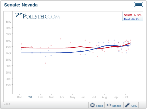
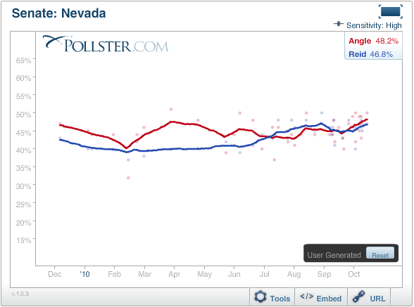
As I explained previously, our standard lines are a smoothed version of the more jagged (and sensitive) lines generated by the Kalman Filter that I have reproduced below. These currently also show Angle leading by a 1.4 percentage point margin (48.2% to 46.8%). The pure Kalman Filter chart can be seen by clicking using the Tools in the interactive version of the chart, clicking the "Smoothing" tool and choosing the "More Sensitive" option.
The Kalman Filter model can do more than produce these trend lines. As we noted last week, the model employs a commonly used technique called Forward Filtering Backward Sampling (FFBS) (Kim, Shepherd, and Chib, 1998) to smooth our results. Among other things, the technique allows the model to make use of all available polling data -- including evidence of global trends seen across all races -- to estimate how the trend line will move from the day of the last poll to Election Day.
A little more information for the statistical gurus (mere mortals can skip to the next paragraph): FFBS takes the estimated means (i.e., the estimated support for a candidate on any given day) and covariances (i.e., how much the support for each candidate is moving around on its own and as a function of other races) from the Kalman filter and then re-estimates the support on a given day T based on what happened on day T+1 (for those interested we're just sampling from a multivariate normal with mean and covariance estimated by the Kalman filter). In order to refine the estimates, the forward filtering part runs the Kalman filter forward from Day 1 to election day, and the backward sampling part runs multivariate normal sampling backwards from election day to Day 1. This process not only smooths our results, but can also be iterated multiple times to get many "simulations" of what happens between Day 1 and election day. The means of these simulations are used for our estimates of support, and the multiple simulations can be used to estimate the probability that a candidate will win a race.
Here's an illustration of the way the FFBS process extends the trend lines in Nevada. In this case, both the Angle and Reid lines move upward over the last two weeks of the campaign (the last poll was completed on October 17), but the margin between them stays roughtly the same. That trend is more than plausible -- the small number of undecideds is shrinking as voters make up their minds.
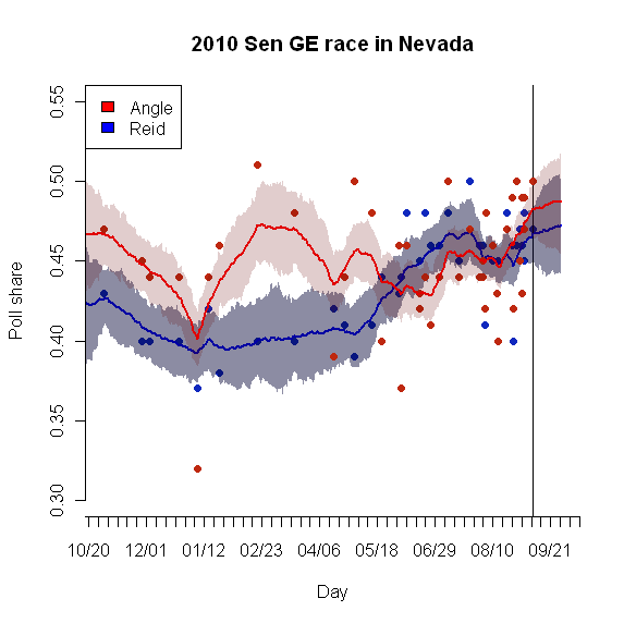
As implied by the bands of light red and light blue ("confidence intervals") drawn around each line, these trend lines can be used to generate probabilities that the leader is actually ahead at any point of the line, including Election Day. For the most competitive races, where polling has been frequent and the most recent polls are only a few days old, the model predicts an Election Day margin that is virtually identical to the last-day-of-the-last-poll trend estimate.
However, in the contests where leads have been bigger and polls less frequent, the time lapse between the last poll and Election Day is longer, and the forward-filtering can alter the leader's projected margin to a greater degree. Because we know that Kalman-Filtering has its limitations, like any other statistical technique (some of which are described in Green, Gerber and De Beoff, 1999), we opted not to place complete trust in the Election Day estimate. Instead, the "win probabilities" are really more accurately described as a cross between lead and win probabilities. They represent an average of the probabilities that the current leader is ahead at (1) the end date of the last poll and (2) Election Day. We believe this approach better serves our goal of helping readers put the current polling trend estimates in better perspective.
The final step in our procedure is to weight back the portion of the probability over 50% so that no probability exceeds 95%. That is a fairly unorthodox, ad hoc step that deserves more explanation.
The basic issue is that since our model can effectively pool data across multiple surveys, relatively small leads translate into highly probable outcomes. We found that leads of 7 or more percentage points usually translate into win probabilities of 98% or better, and leads of 8 or more almost always produce 100% certainty about the winner. So long as statewide and Congressional district polling numbers remain unbiased (in the statistical sense), as they have been for at least the last decade, such probabilities are probably about right. Nate Silver, who examined this issue in exhaustive detail recently, finds that no regular, general election Senate candidate "with a lead of more than 5.5 points in the polling average, with 30 days to go in the race, has lost since 1998: these candidates are 68-0. "
Nevertheless, my pollster training leaves me uncomfortable implying 100% confidence in any poll generated estimate, especially in an era where response and coverage rates are a long, long way from optimal. Pollsters have a particular obligation, as spelled out the in ethical code of the American Association for Public Opinion Research (AAPOR), to "be mindful of the limitations of our techniques" and to avoid interpreting the data in way that imply "greater confidence than the data actually warrant." While public polling's past performance may well warrant very high confidence, I believe we do it a disservice by implying 100% certainty that polling is bullet-proof.
Our statistical model assumes no bias in the forecast, no skew due to low response rates, poor coverage due to cell phones and error in the estimation of the likely electorate. Yes, polling over the last 10 to 15 years often shows considerable variability within individual races, that averages typically show little or no bias. The odds are good that this year's polling will be the same, and if so, our probabilities are good-to-go. But unbiased polling this year is not a certainty. Relatively new challenges, such as the recent exponential growth in both cell-phone-only households and early voting, may be creating new problems that our past experience cannot predict.
As such, we made a decision to simply weight back the probabilities, so that our certainty about any race is never greater than 95%. While admittedly arbitrary, this adjustment is party neutral -- it has zero impact on whether any given candidate is considered a leader because the weight decreases to zero as probabilities approach 50%.** Consider this an admission that our probabilities are something of a "beta" version. We look forward to incorporating elegant means of anticipating the real uncertainty in future versions of the model.
As you will see, this adjustment still leaves considerable certainty about the outcome of most races. In 25 of the 36 Senate races for which polling is available, our model gives the leader the maximum 95% win probability, a level that we will use to characterize leads as "strong." In Senate and Governor races, probabilities greater than 75% but less than 95% will be designated as "leaning" to the leader and anything under 75% will constitute a "toss-up." It's important to remember that the dividing lines between these categories is fairly arbitrary -- ultimately the percentages are more important than the line between "toss-up" and "lean."
Even with the weight applied, you will see that relatively modest leads on our trend estimate can easily approach 75%. In Nevada, for example, Sharon Angle's 1.3 percent lead translates into a 72% win probability (as of this writing), just a few points below "lean" status.
But keep in mind that a 75% win probability means there is still a one-in-four chance that the trailing candidate might win. In 2008, our final trend estimates showed margins under two percentage points in seven races: The race for president in Florida, Missouri, Indiana, North Carolina and North Dakota, the Senate race in Minnesota and the Governor's race in North Carolina. Despite these very narrow margins, the leader in the polling averages lost in only two of the seven cases -- pretty close to what our weighted model probabilities predict.
The model for the House races is a bit more complex -- and interesting -- and I will describe that in a subsequent post.
**We weighted down probabilities as follows: where P is the original probability (a number between 0 and 100), and PW is the new weighted probability: PW = [(P-50)*0.9)]+50